 Python-based
Hierarchical
ENvironment
for
Integrated
Xtallography
Python-based
Hierarchical
ENvironment
for
Integrated
Xtallography
At low resolution there are far fewer diffraction spots than there are atomic coordinates to determine. The data alone cannot fully determine the model, so we lean on prior chemical and structural knowledge, encoded as restraints, to keep the model sensible. This tutorial walks through the restraints that matter most at low resolution and shows, with real numbers, what each one contributes:
The same ideas apply to cryo-EM refinement in phenix.real_space_refine; here we use X-ray data because R-free provides an independent cross-validation score.
Everything below is presented through the phenix.refine GUI. Each step also lists the equivalent command line, and the full set of commands is collected at the end. You may find the dictionary of terms helpful.
Set up the example in the GUI as described here. In the tutorial setup window, select the dataset labeled "Low resolution restraints (2h1g/2f9s)" under "Refinement", and click "Okay". Once the project is created, click the button labeled "phenix.refine" in the main GUI under "Refinement".
Add the starting model 2h1g.pdb and the reflections 2h1g-sf.mtz to the input file list. The space group and unit cell load automatically. For the reference-model step (Step 2) you also add reference_2f9s.eff, which defines the reference-model restraints and points at the two reference_for_chain_*_2F9S.pdb files; alternatively you can add those two PDB files directly and tag them as "Reference model".
After each run, look at these, printed at the end of the phenix.refine log and by phenix.molprobity:
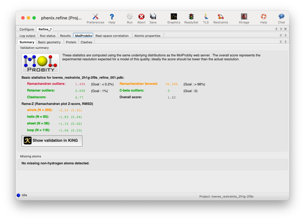
The GUI reports clashscore, Ramachandran, rotamer, MolProbity score and Rama-Z on the MolProbity results tab after each run:
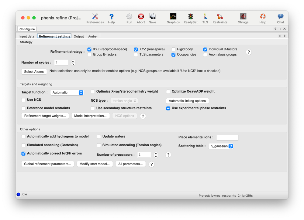
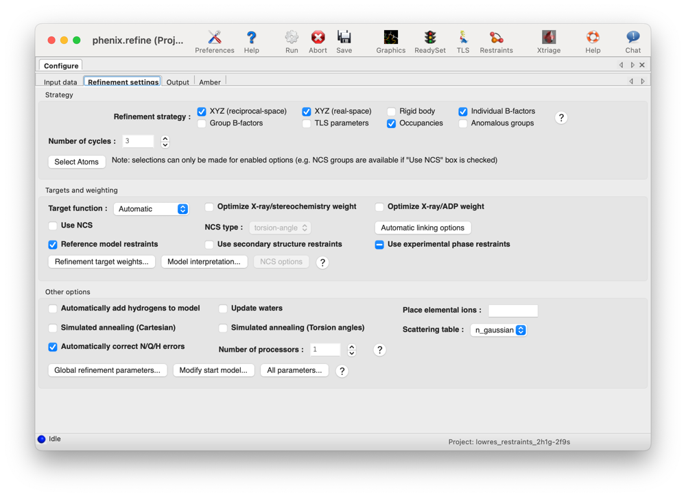
Most restraint options live in one place: the Refinement settings tab, "Targets and weighting" section. The "Use NCS" checkbox and NCS type, the "Reference model" checkbox, and the "Secondary structure" checkbox are all here; the finer parameters sit behind the "Model interpretation..." button in the same section.
First, look at the model as it was deposited, before refining anything. Run phenix.molprobity on the deposited 2h1g.pdb against 2h1g-sf.mtz (and mmtbx.rama_z 2h1g.pdb for Rama-Z):
R-work 0.1857   R-free 0.2446   gap 0.0589
clashscore 8.9   Rama favored 93.7%   Rama outliers 1.49%   rotamer outliers 6.7%
MolProbity 2.52   Rama-Z -2.93  (poor)
That is a 3.10 A model with a MolProbity near 2.5 and a Rama-Z deep in the "poor" band. Now run a plain refinement with no extra restraints.
In the GUI: in the Refinement settings tab, Targets and weighting section, leave every restraint box unchecked (Reference model, Secondary structure and Use NCS all off) and click Run:
R-work 0.1349   R-free 0.2281   gap 0.0932
clashscore 6.8   Rama favored 96.3%   Rama outliers 1.49%   MolProbity 1.62
Rama-Z -2.53  (suspicious)
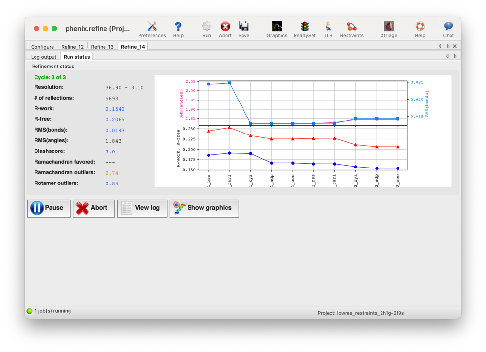
R-work is 0.1349 but R-free is 0.2281. With ~5700 reflections and ~2170 atoms there are barely more observations than parameters, so the model over-fits. Closing that gap is what the restraints below are for. The Run status tab plots R-work and R-free over the macro-cycles, so you can watch the gap directly.
In the GUI: in Refinement settings -> Targets and weighting, tick the Secondary structure checkbox. (Fine control and hand-curated annotations live behind the Model interpretation... button, under secondary_structure.)
phenix.refine finds the helices and sheets automatically and adds explicit hydrogen-bond distance restraints; the log lists the elements it restrains and any outlier H-bonds it rejects.
R-work 0.1398   R-free 0.2274   gap 0.0876
clashscore 7.0   Rama favored 94.8%   Rama outliers 1.49%   MolProbity 1.74
Rama-Z -2.12
On its own, automatic SS finding barely moves R-free here. Its value is as a safeguard against helices unwinding during refinement, and in combination with the other restraints (Step 2).
Command line:
phenix.refine 2h1g.pdb 2h1g-sf.mtz \
    refinement.pdb_interpretation.secondary_structure.enabled=True
If a higher-resolution structure of the same protein exists, we can restrain our model's torsion angles toward it -- borrowing the well-determined geometry of the 1.40 A structure (2f9s) to guide our 3.10 A model.
In the GUI: add reference_2f9s.eff to the Input files list, then tick the Reference model checkbox in Targets and weighting. In the log, find the "Reference Model Matching Summary" (about 1228 torsion restraints here).
R-work 0.1497   R-free 0.2122   gap 0.0625
clashscore 4.9   Rama favored 99.3%   Rama outliers 0.74%   MolProbity 1.26
Rama-Z 0.33   (good)
R-free drops from 0.2281 to 0.2122, the gap shrinks, MolProbity improves from 1.62 to 1.26, and Rama-Z moves from -2.53 into the "good" band at 0.33.
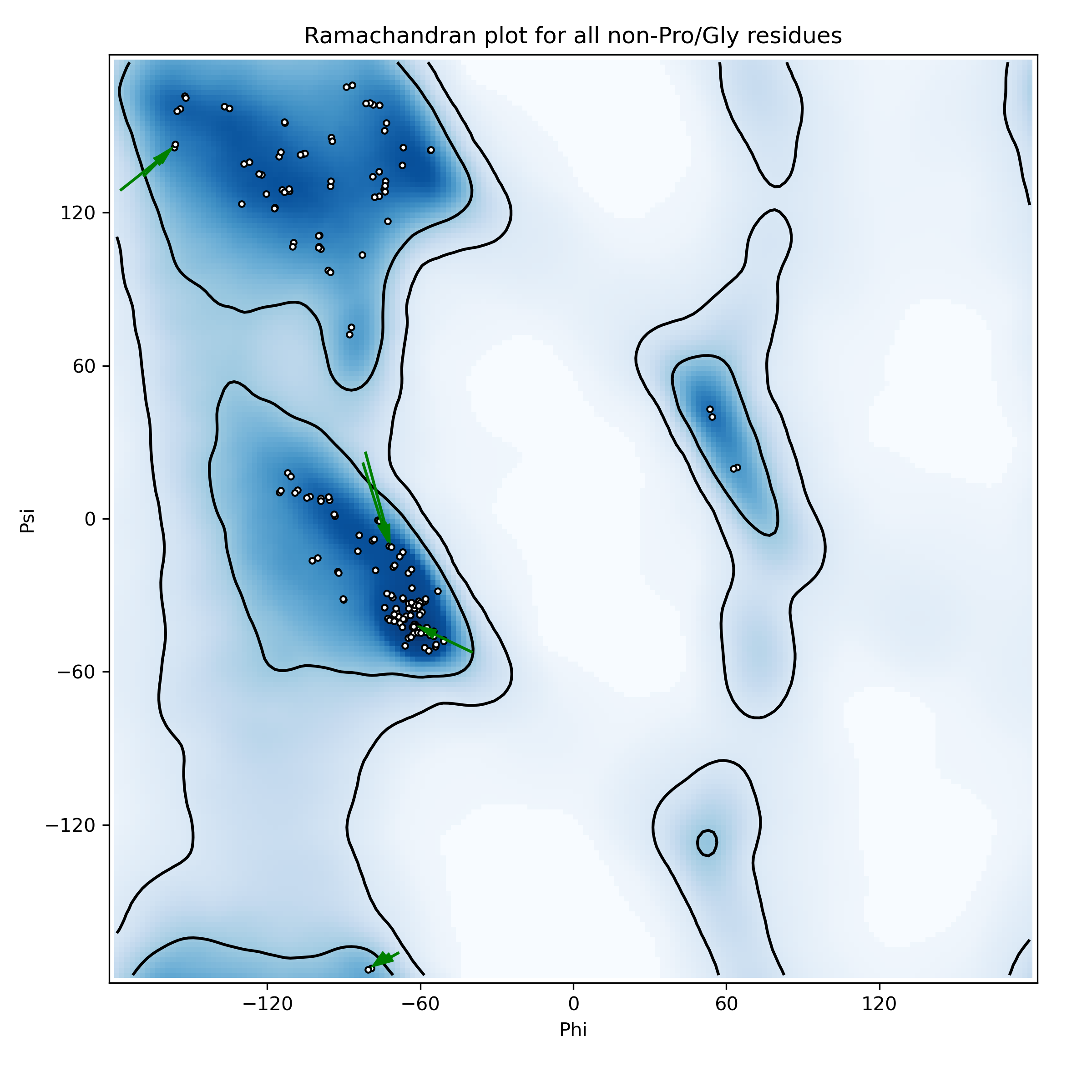
phenix.comparama, deposited model to reference-model run. Fifteen residues climb into the favoured region (green arrows) and not one gets worse -- each residue is pulled toward the geometry of its high-resolution counterpart, so it lands where it belongs. This is the visual counterpart of the R-free and Rama-Z improvement.
Command line:
phenix.refine 2h1g.pdb 2h1g-sf.mtz reference_2f9s.eff
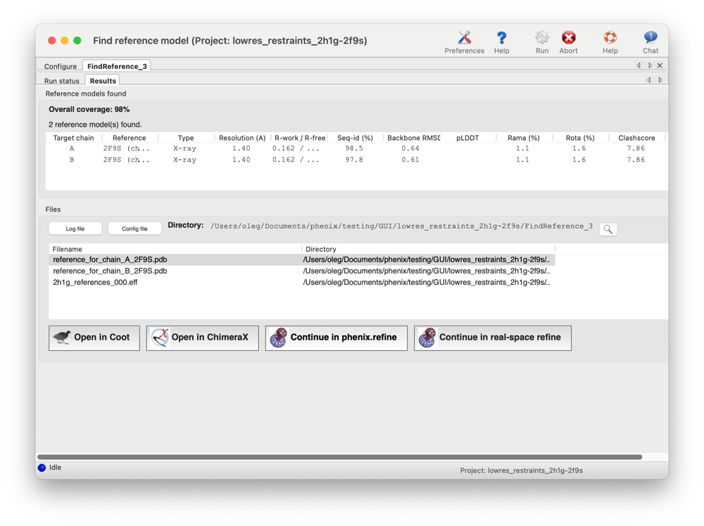
Where the reference came from (optional). The shipped reference files let Step 2 run with no internet and reproduce the numbers above. To build your own instead, use phenix.find_reference on 2h1g.pdb: it searches the PDB, ranks 2F9S first, trims and superposes a copy onto each chain, and writes the reference PDBs and .eff. In the GUI, the phenix.find_reference results panel has a "Continue in phenix.refine" button that carries the whole reference-model setup straight into refinement.
A live search needs internet, and because the PDB keeps growing it may rank a different structure or superpose it slightly differently, so your R-free may not match the table to the last digit -- the shipped files are the reproducible version. Note also that using the raw deposited 2f9s.pdb directly restrains only chain A (~722 restraints); the find_reference output supplies one reference group per target chain, so both chains are restrained (~1228 restraints, R-free 0.2122).
The two copies (chains A and B) should be nearly identical, so we can tie them together.
In the GUI: tick Use NCS in Targets and weighting, then set the NCS type drop-down to torsion-angle (or constraints). The residue_match_radius control sits behind the Model interpretation... button, under ncs_search (see below).
Torsion NCS (recommended). Ties the torsion angles of matching residues while letting the copies differ in position where they actually differ:
R-work 0.1426   R-free 0.2234   gap 0.0808
clashscore 5.6   Rama outliers 0.74%   MolProbity 1.52   Rama-Z -2.13
NCS constraints (strict -- handle with care). Constraints force the copies to be identical:
R-work 0.1673   R-free 0.2486   gap 0.0813
clashscore 7.9   Rama outliers 0.74%   MolProbity 1.71   Rama-Z -2.27
Forcing the copies to be identical makes both R-work and R-free go up and the clashscore worse. The copies are similar but not identical, so prefer torsion NCS at low resolution.
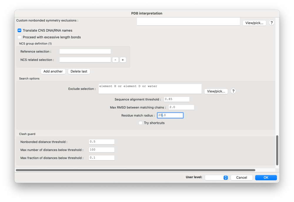
Which residues are "the same"? Whichever land within residue_match_radius of each other after superposition (default 4.0 A); residues that diverge more are excluded from the NCS group. This control is behind the "Model interpretation..." button, under ncs_search.
In 2h1g the backbone of the two copies overlaps closely; at the default 4.0 A radius just two surface residues per chain are excluded -- Lys79 (side-chain tips ~5.1 A apart) and His111 (imidazole tips ~4.4 A apart). Loosening the radius to 10 A pulls them back into the group and forces them to match. The illustrations folder shows these two residues; you can reproduce the view live in Coot with NCS ghosts.
Command line:
phenix.refine 2h1g.pdb 2h1g-sf.mtz \
    refinement.pdb_interpretation.ncs_search.enabled=True \
    refinement.ncs.type=torsion        # or =constraints
These push each residue's backbone phi/psi toward the favoured regions of the Ramachandran plot.
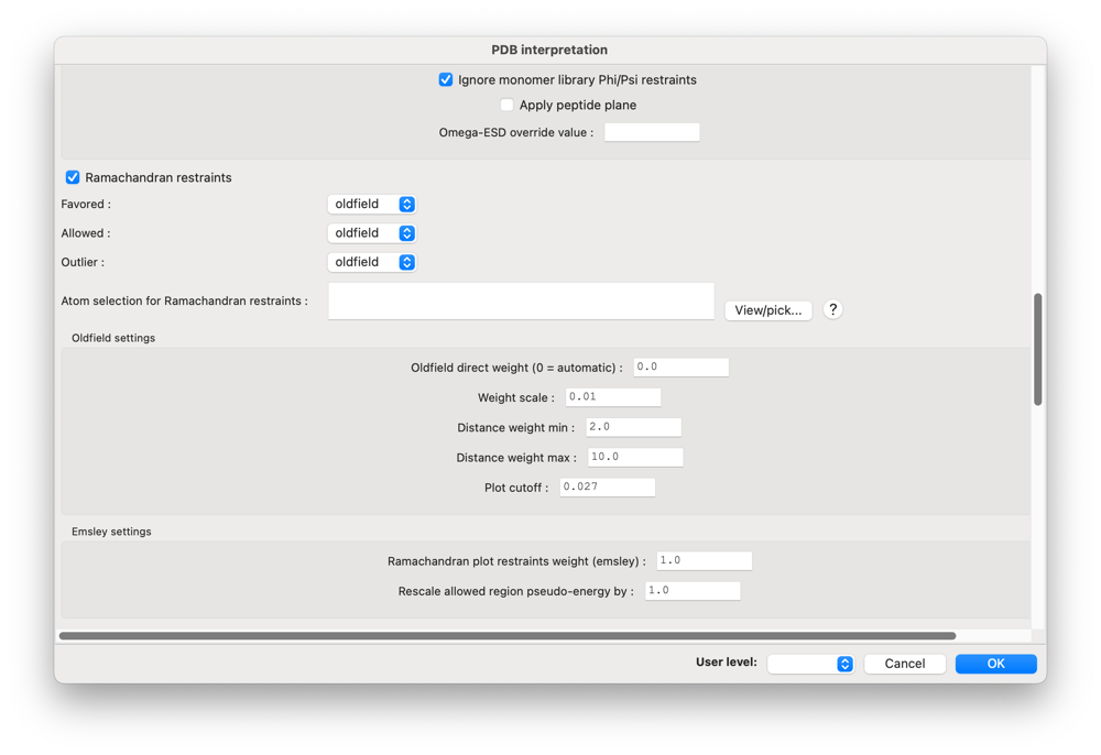
In the GUI: there is no top-level checkbox for this one -- click Model interpretation... in Targets and weighting and tick Ramachandran restraints (ramachandran_plot_restraints).
R-work 0.1367   R-free 0.2259
clashscore 7.0   Rama outliers 0.00%   Rama favored 96.3%   MolProbity 1.64
Rama-Z -1.38
Ramachandran restraints drive outliers to zero (1.49% -> 0.00%), which looks great, but be careful why. They push each residue into the nearest favoured region, which may not be the correct one. R-free barely moves (0.2281 -> 0.2259) and Rama-Z reaches only -1.38, worse than the reference-model result (0.33). Use them as a finishing touch on an already-good model, not to make a bad one look good.
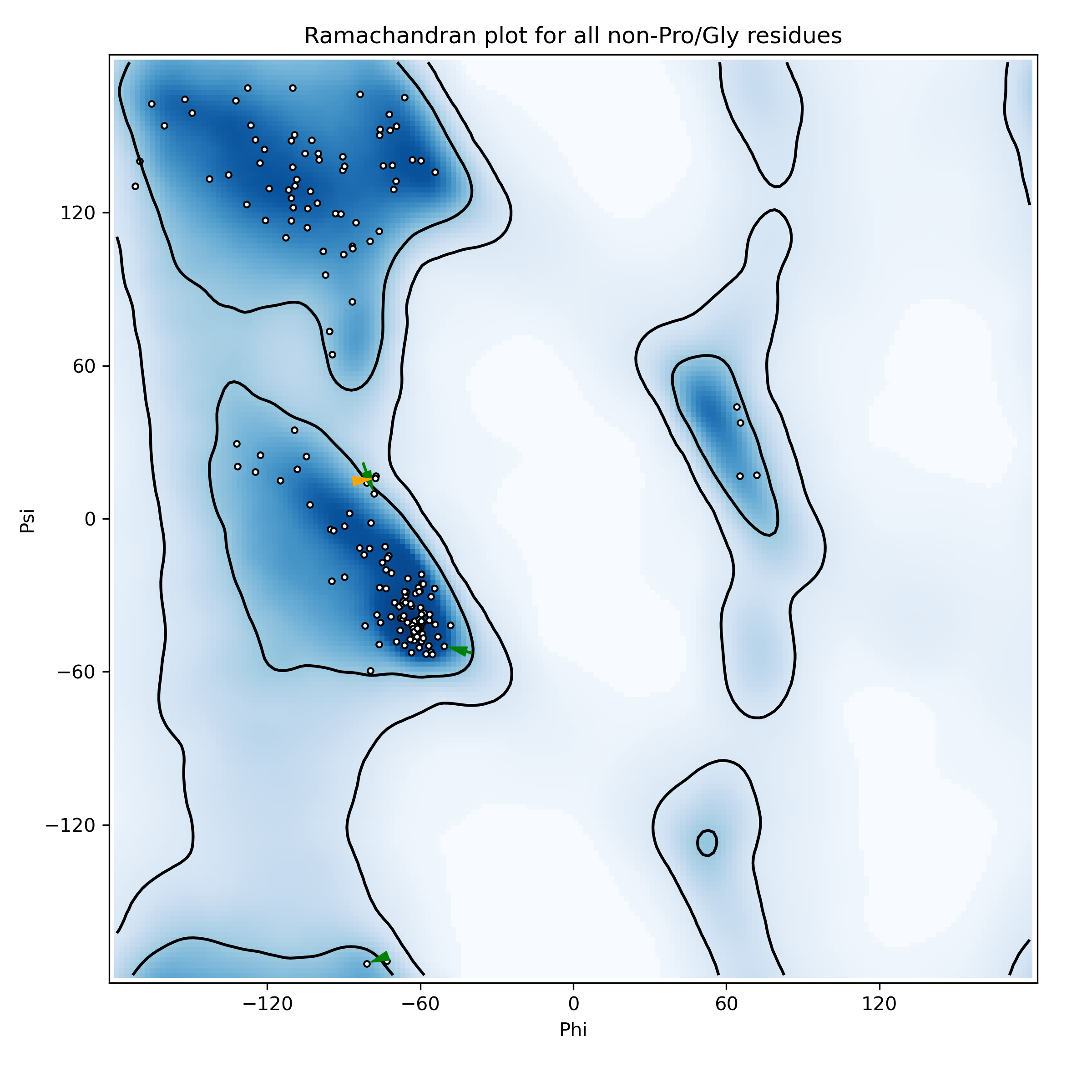
phenix.comparama, deposited model to Ramachandran-restraint run. Every outlier is cleared, but several arrows stop in the "allowed" band rather than "favoured", and one favoured residue slips to allowed: the restraints shove each residue into the nearest region, not necessarily the correct one. Compare the reference-model plot in Step 2, where the arrows carry residues all the way into favoured -- that is why the reference run lowers R-free and Rama-Z while this one barely moves them even though the outlier count reads zero.
If you have a good reference you can instead use its actual phi/psi as the Ramachandran targets (a sub-option of the reference-model restraints, reference_model.ramachandran_targets). This path is command-line/PHIL only and requires two extra flags:
phenix.refine 2h1g.pdb 2h1g-sf.mtz reference_2f9s.eff \
    refinement.reference_model.ramachandran_targets.enabled=True \
    refinement.pdb_interpretation.ramachandran_plot_restraints.enabled=True \
    refinement.pdb_interpretation.ramachandran_plot_restraints.inject_emsley8k_into_oldfield_favored=False
Because the targets are real phi/psi from a genuine structure rather than "nearest favoured", it is less prone to pushing residues into the wrong region.
The restraints are complementary. Combining reference-model + secondary-structure + torsion NCS gives the best all-round result here.
In the GUI: tick Reference model, Secondary structure and Use NCS (NCS type = torsion-angle) together in Targets and weighting:
R-work 0.1519   R-free 0.2020   gap 0.0501
clashscore 4.4   Rama favored 99.3%   Rama outliers 0.74%   MolProbity 1.22
Rama-Z 0.76   (good)
R-free has gone from 0.2281 (default) to 0.2020, and MolProbity from 1.62 to 1.22. As a finishing touch you can add generic Ramachandran restraints on top of this combination (tick Ramachandran restraints in the Model interpretation dialog as well): on an already-good model they do no harm and cut the remaining Ramachandran outliers from 0.74% to 0.37% at essentially no cost in R-free (0.2020 -> 0.2025).
scenario           Rwork   Rfree   gap    | clash ramaOut ramaFav MPscore Rama-Z
-------------------------------------------------------------------------------
START (deposited)  0.1857  0.2446  0.0589 |  8.9   1.49    93.7    2.52   -2.93
default            0.1349  0.2281  0.0932 |  6.8   1.49    96.3    1.62   -2.53
+ SS               0.1398  0.2274  0.0876 |  7.0   1.49    94.8    1.74   -2.12
+ reference        0.1497  0.2122  0.0625 |  4.9   0.74    99.3    1.26    0.33
+ NCS torsion      0.1426  0.2234  0.0808 |  5.6   0.74    96.7    1.52   -2.13
+ NCS constraints  0.1673  0.2486  0.0813 |  7.9   0.74    95.9    1.71   -2.27
+ Ramachandran     0.1367  0.2259  0.0892 |  7.0   0.00    96.3    1.64   -1.38
ALL (ref+SS+NCS)   0.1519  0.2020  0.0501 |  4.4   0.74    99.3    1.22    0.76
ALL + Ramachandran 0.1519  0.2025  0.0506 |  4.7   0.37    99.3    1.24    0.93
A single number (Rama outliers %) hides which residues changed and whether they moved to the right place. phenix.comparama draws a Kleywegt-style Ramachandran plot with an arrow from each residue's before phi/psi to its after phi/psi, coloured by what happened (green = moved into favoured, orange = favoured to allowed, red = moved into outlier):
phenix.comparama 2h1g.pdb 2h1g_refine_001.pdb output.plots=True
It also prints a text summary counting every transition. Across all steps (deposited model -> refined model):
scenario            improved   made worse   outliers left
---------------------------------------------------------
default                 8          2             4
+ SS                    8          5             4
+ reference            15          0             2   <-- best
+ NCS torsion           9          0             2
+ NCS constraints       9          2             2
+ Ramachandran         12          1             0
ALL (ref+SS+NCS)       15          0             2
ALL + Ramachandran     16          0             1
The plots for every step of this tutorial are in the illustrations/comparama folder (comparama_<step>.png, and *_allplots.pdf for the per-residue-class breakdown), all computed as deposited-model to refined-model so they are directly comparable. The two plots above make the key contrast: the reference-model run (Step 2) moves 15 residues into favoured with none getting worse, while the Ramachandran-only run (Step 4) clears every outlier but leaves several residues stuck in the "allowed" band. Combining the restraints keeps the clean behaviour of the reference run:
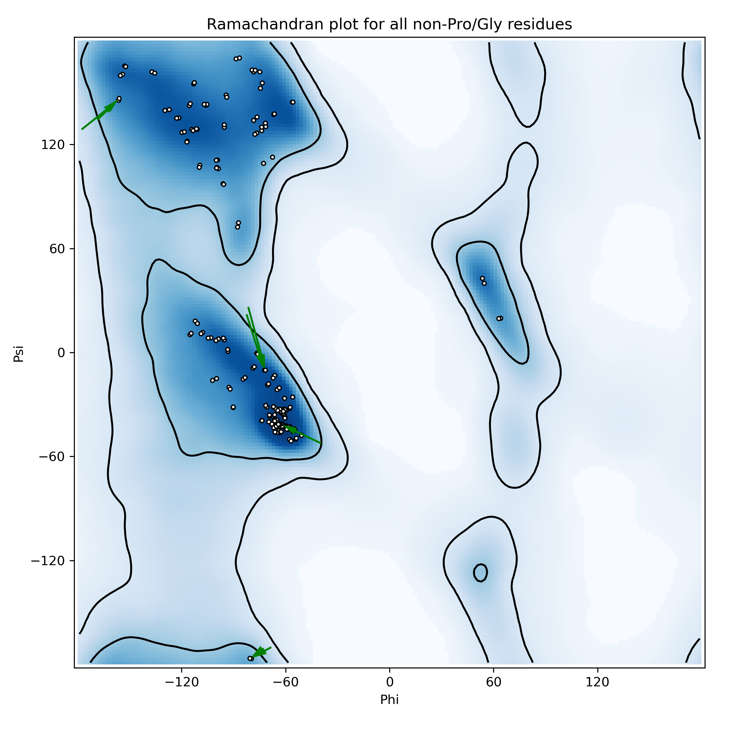
phenix.comparama for the combined run (reference model + secondary structure + torsion NCS): the arrows climb into the dense favoured regions, matching its best-in-table R-free (0.2020) and MolProbity (1.22).
Step 0  phenix.refine 2h1g.pdb 2h1g-sf.mtz
Step 1  phenix.refine 2h1g.pdb 2h1g-sf.mtz \
            refinement.pdb_interpretation.secondary_structure.enabled=True
Step 2  phenix.refine 2h1g.pdb 2h1g-sf.mtz reference_2f9s.eff
Step 3a phenix.refine 2h1g.pdb 2h1g-sf.mtz \
            refinement.pdb_interpretation.ncs_search.enabled=True refinement.ncs.type=torsion
Step 3b phenix.refine 2h1g.pdb 2h1g-sf.mtz \
            refinement.pdb_interpretation.ncs_search.enabled=True refinement.ncs.type=constraints
Step 4  phenix.refine 2h1g.pdb 2h1g-sf.mtz \
            refinement.pdb_interpretation.ramachandran_plot_restraints.enabled=True
Step 5  phenix.refine 2h1g.pdb 2h1g-sf.mtz reference_2f9s.eff \
            refinement.pdb_interpretation.secondary_structure.enabled=True \
            refinement.pdb_interpretation.ncs_search.enabled=True refinement.ncs.type=torsion